1.2.1. Sources

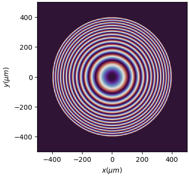
One main part of this software is the generation of optical fields such as:

• Plane waves.

• Spherical waves.

• Gaussian beams.

• Bessel beams.

• Vortex beams.

• Laguerre beams.

• Hermite-Gauss beams.

• Zernike beams

• …

1.2.2. Masks

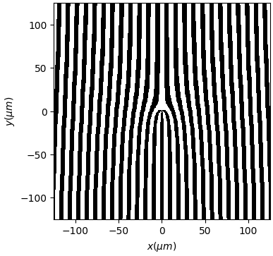
Another important part of Diffractio is the generation of masks and Diffractive Optical Elements such as:

• Slits, double slits, circle, square, ring …

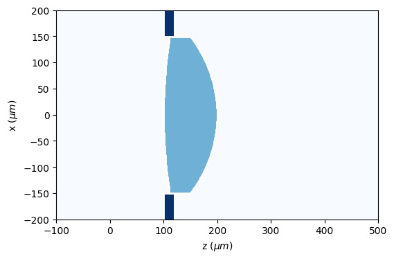
• Lenses, diffractive lenses, aspherical lenses…

• Axicon, prisms, biprism, image, rough surface, gray scale …

• Gratings: Ronchi, phase, radial, angular, sine, forked, blazed, 2D, chess…

• From files: Masks can also be loaded (.png, .dxf for 2D and .stl for 3D).

• …

In the XZ scheme there is also a number of masks:

• image, cylinder, layer, lenses, wedge, prism, probe, gratings…

• Additionally, any X_mask can be extruded to the XZ scheme.

• Masks from functions.

• Surfaces can be added to objects.

1.2.3. Propagation algorithms

Several propagation algorithms for propagation of light are implemented in the fields modules:

The main algorithms for Scalar propagation are:

• Fast Fourier Transform (FFT) which allows, in a single step, to determine the field at the far field.

• Rayleigh-Sommerfeld (RS) [Appl. Opt., 45(6) 1102–1110, (2006)] RS allows, in a single step, to propagate to a near or far observation plane, which allows fast computations. The fields and the masks must be defined in a plane.

• Plane Wave Decomposition (PWD) [Opt. Comm. 281 4219-4233 (2008)] PWD allows to propagate to a near or far observation plane. It presents a complexity of O(n) in the two-dimensional and O(n2) in the three-dimensional case. It is computed according to the split-step propagation scheme.

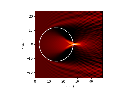
• Beam propagation method (BPM) [Appl. Opt. 24, 3390-3998 (1978)] which allows to analyze the propation of light in volumetric elements, such as spheres, cylinders and other complex forms, provided that the spatial variations in the refractive index are small. It allows graded index structures. It presents a complexity of O(n) in the two-dimensional and O(n2) in the three-dimensional case. It is computed according to the split-step propagation scheme.

• Wave Propagation Method (WPM). [Appl. Opt. 32, 4984 (1993)] WPM was introduced in order to overcome the major limitations of the beam propagation method (BPM). With the WPM, the range of application can be extended from the simulation of waveguides to simulation of other optical elements like lenses, prisms and gratings. WPM can accurately simulate scalar light propagation in inhomogeneous media at high numerical apertures, and provides valid results for propagation angles up to 85° and that it is not limited to small index variations in the axis of propagation. Fast implementation with discrete number of refractive indexes is also implemented.

• Chirped Z-Transform (CZT). [Light: Science and Applications, 9(1), (2020)] CZT allows, in a single step, to propagate to a near or far observation plane. It present advantages with respecto to RS algorithm, since the region of interest and the sampling numbers can be arbitrarily chosen, endowing the proposed method with superior flexibility. CZT algorithm allows to have a XY mask and compute in XY, Z, XZ, XYZ schemes, simply defining the output arrays.

1.2.4. Other features

• When possible, multiprocessing is implemented for a faster computation.

• The fields, masks, and sources can be stored in files.

• Also drawings can be easily obtained, for intensity, phase, fields, etc.

• In some modules, videos can be generated for a better analysis of optical fields.

• Intensity, MTF and other parameters are obtained from the optical fields.

• Fields can be added simply with the + signe, and interference is produced. Masks can be multiplied, added and substracted in order to make complex structures

• Resampling fields in order to analyze only areas of interest.

• Save and load data for future analysis.

• Rayleigh-Sommerfeld implementation is performed in multiprocessing for fast computation.

• Polychromatic and extended source problems can also be analyzed using multiprocessing.

1.3.1. Sources

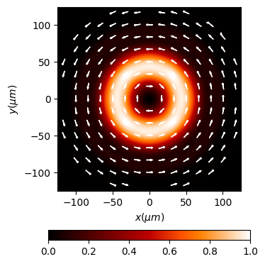
Vector sources as implemented in vector_sources_XY module.

The can present any spatial distribution of the electric field, and can be defined in the XY plane.

In addition, the polarization state is defined by the Jones vector, which can be constant (linear, circular, elliptical) or spatially varying, such as (azimuthal, radial, spiral, etc.).

• constant_polarization.

• azimuthal_wave, azimuthal_inverse_wave.

• radial_wave, radial_inverse_wave.

• local_polarized_vector_wave, local_polarized_vector_wave_radial, local_polarized_vector_wave_hybrid.

• spiral_polarized_wave.

1.3.2. Masks

Vector masks are defined in the vector_masks_XY module by Jones matrices.

For example, a scalar mask is transformed to a vector mask by applying a Jones matrix to the scalar mask (scalar_to_vector_mask).

There are also predefined vector masks for standard polarizers (linear, quarter-wave, half-wave). Arbitrary Jones matrices can be defined for any mask using from_pypol method.

Binary scalar masks can also be transformed to vector masks using two Jones matrices (complementary_masks).

Also, arbitrary vector masks can be defined by defining the Jones matrix for each index level. This can be used for defining Spatial Light Modulators (SLM).

Here, we implement new classes where the E_x, E_y, and E_z fields are generated and propagated using Rayleigh-Sommerfeld and Chirped z-transform algorithms. Also, simple and complex polarizing masks can be created.

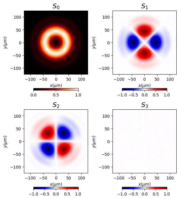
Intensity of vector field

Polarization: Stokes parameters

1.3.3. Propagation algorithms

The main algorithms for Vector propagation are:

• Vector Fast Fourier Tranform (VFFT), which allows to determine the (Ex, Ey, Ez) fields at the far field.

• Vector Rayleigh-Sommerfeld (VRS). The VRS method [Laser Phys. Lett. 10(6) 065004 (2013)] allows to propagate (Ex,Ey,Ez) fields offering the advantage of significant reduction in computation, from flat diffractive elements (Thin Element Approximation) with full control of polarization. It addresses simultaneously both longitudinal polarization. This approach offers the advantage of significant reduction in computation.

• Vector Chirp Z-Transform (VCZT). [Light: Science and Applications, 9(1), (2020)]. CZT is also implemented in vector fields.

• Fast Polarized Wave Propagation Method (FP_WPM) [Opt Express. 30(22) 40161-40173 (2022)] Wave Propagation Method for vector fields. It is an efficient method for vector wave optical simulations of microoptics. The FPWPM is capable of handling comparably large simulation volumes while maintaining quick runtime. By considering polarization in simulations, the FPWPM facilitates the analysis of optical elements which employ this property of electromagnetic waves as a feature in their optical design, e.g., diffractive elements, gratings, or optics with high angle of incidence like high numerical aperture lenses.

1.3.4. Other features

Vector fields can be converted to py-pol objects for further analysis.